Benchmarking AutoML for Time Series Forecasting

A comparison of AutoML to Prophet and sktime.

Over the past year, I have been developing a Python package for automated machine learning (AutoML). While I mainly use the package for standard supervised learning, I have recently begun using it for time series. The workflow is the same: fitting several models and selecting the model with highest out-of-sample accuracy.

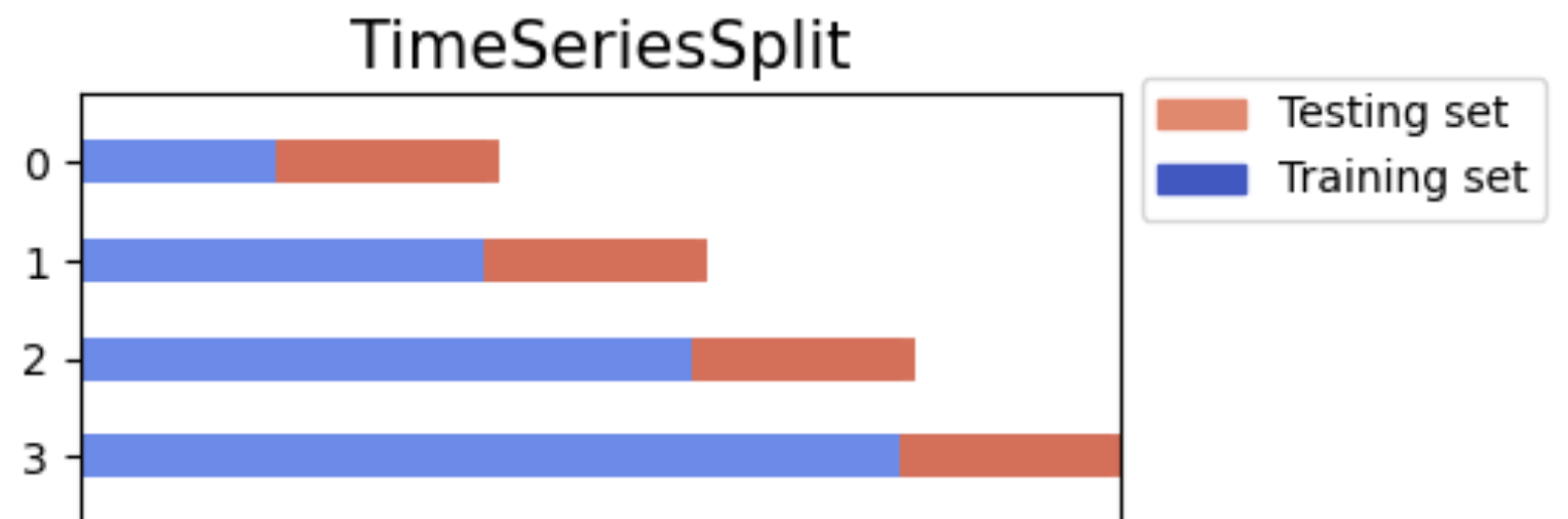
However, the time series mode of the package has a few differences. First, instead of standard k-fold cross-validation, the time series mode uses TimeSeriesSplit from scikit-learn. Rather than partitioning the data into random folds, TimeSeriesSplit uses an expanding window. Each CV iteration evaluates on a test set that follows the training set, while the training set grows to include all prior data:

The other difference with time series mode is the use of automated feature engineering. The tool generates several transformations of the dependent variable – lags, rolling averages, and cyclical features (sine transformations for seasonality) – to use as predictors. My hypothesis was that training ElasticNet and gradient boosting models on these engineered features would yield accurate forecasts. This approach is based in part on my experience with enterprise AutoML platforms like DataRobot, which use a similar methods.

Finally, the time series mode of my tool includes classical statistical models such as Exponential Smoothing and ARIMA that ignore the transformed features and model the original series directly.

Benchmarking AutoML against Prophet and sktime

To benchmark my tool, I compared AutoML to Facebook Prophet and a comprehensive set of models from the sktime library.

I used a variety of datasets, including real-world series from the Federal Reserve Economic Database (unemployment rate, the consumer price index, industrial production), synthetic datasets (linear trends, quadratic and logistic functions), and a sample atmospheric CO2 dataset from statsmodels.

You can find the notebook showing how the data was created and the models were trained here.

Here is a table comparing mean absolute errors (MAEs) for each framework. These were calculated using a rolling one-step ahead forecast over a holdout set comprising the final 24 periods of each time series.

Series	Type	AutoML MAE	Prophet MAE	sktime MAE	Winner
Seasonal+Trend	Synthetic	1.76	1.91	1.57	sktime
Linear Trend	Synthetic	2.18	2.23	2.15	sktime
Quadratic	Synthetic	1.54	12.32	1.44	sktime
Logistic (S-curve)	Synthetic	2.50	2.87	2.32	sktime
Random Walk (drift)	Synthetic	0.72	1.69	1.48	automl
Piecewise (changepoints)	Synthetic	1.92	1.91	2.97	prophet
Spiky Intermittent	Synthetic	1.67	1.64	1.66	prophet
Multi-seasonal	Synthetic	1.46	1.40	1.58	prophet
CO2	Real (statsmodels)	0.25	0.37	0.29	automl
CPIAUCSL	Real (FRED)	0.44	1.53	2.90	automl
UNRATE	Real (FRED)	0.12	0.28	0.17	automl
INDPRO	Real (FRED)	0.46	0.72	1.66	automl
Average		1.25	2.41	1.68	automl

Among these time series, AutoML outperformed the other tools on real world data. sktime and Prophet did better on the synthetic functions, but even on these AutoML wasn’t far behind. This is reflected in the average MAE: AutoML had an average MAE of 1.25, compared to 1.68 for sktime and 2.41 for Prophet.

Which models did AutoML favor?

The table below shows the winning model for each time series and framework (check out my introduction AutoML post to learn how to use the package).

import pandas as pd

(pd.read_csv('input_data/combined_performance.csv')
 [['series', 'automl_winner', 'prophet_winner', 'sktime_winner']]
 .rename(columns=lambda x: x.replace('_', ' ').title())
 .dropna()
)

	Series	Automl Winner	Prophet Winner	Sktime Winner
0	Seasonal+Trend	ElasticNet	GAM CPS: 0.005 SPS: 15.0 Seasonality: additive...	XGB-Reduction
1	Linear Trend	SimpleESRegressor	GAM CPS: 0.5 SPS: 5.0 Seasonality: additive Gr...	EnsembleTop3
2	Quadratic	AutoARIMARegressor	GAM CPS: 0.05 SPS: 15.0 Seasonality: multiplic...	Trend2
3	Logistic (S-curve)	ElasticNet	GAM CPS: 0.5 SPS: 15.0 Seasonality: multiplica...	ETS-add-none-sp1
4	Random Walk (drift)	ElasticNet	GAM CPS: 0.5 SPS: 5.0 Seasonality: additive Gr...	ETS-none-add-sp12
5	Piecewise (changepoints)	ElasticNet	GAM CPS: 0.05 SPS: 5.0 Seasonality: additive G...	ETS-add-add-sp12
6	Spiky Intermittent	SimpleESRegressor	GAM CPS: 0.05 SPS: 5.0 Seasonality: multiplica...	ETS-add-add-damped-sp12
7	Multi-seasonal	SimpleESRegressor	GAM CPS: 0.5 SPS: 15.0 Seasonality: multiplica...	RF-Reduction
8	CO2	ElasticNet	GAM CPS: 0.005 SPS: 15.0 Seasonality: additive...	XGB-Reduction
9	CPIAUCSL	ElasticNet	GAM CPS: 0.05 SPS: 15.0 Seasonality: multiplic...	Naive-drift
10	UNRATE	ElasticNet	GAM CPS: 0.005 SPS: 15.0 Seasonality: additive...	EnsembleTop3
11	INDPRO	ElasticNet	GAM CPS: 0.05 SPS: 15.0 Seasonality: additive ...	Naive-last

Most of the best performing models from my AutoML tool are ElasticNet models. AutoML selects the ElasticNet model with the optimal alpha and l1_ratio (ratio of L1 to L2 regularization) terms. For some of the synthetic series, the best models were exponential smoothing and ARIMA.

Prophet models are an implementation of GAMs (generalized additive models) for time series. For each series, I used hyperparameter tuning to select a GAM with the optimal changepoint prior scale, seasonality prior scale, seasonality model, and other hyperparameters.

sktime displayed the greatest variety of winning models. The framework favored exponential smoothing (ETS) for several series. The best sktime models also included ensemble models – random forests (RF-Reduction), gradient boosting (XGB-Reduction), and stacking (EnsembleTop3). Quadratic (Trend2), and rule-based (Naive-last) models were also selected.

The power of ElasticNets for time series

My main takeaway from this exercise, aside from AutoML being a viable alternative to Prophet and sktime for automated time series, is the effectiveness of ElasticNets for time series forecasting. The key is feature engineering. By feeding the model a large array of lagged transformations, the ElasticNet uses the L1 and L2 regularization terms to suppress features with poor predictive power and emphasize the predictive features.

My evaluation focused only on rolling one-period ahead forecasts. However, the AutoML tool can handle forecast windows greater than one. This is specified by the forecast window parameter. The next step in this analysis will be to determine how AutoML compares to Prophet and sktime at forecasting multiple periods out.

Finally, the time series mode of the AutoML tool currently only handles univariate analysis. In a future version of the package, I plan to add support for time series with exogenous variables (e.g., modeling unemployment on multiple FRED economic indicators).